Stability and Transcritical Bifurcation of a Discrete Predator-Prey Model with Predator Cannibalism
Received Date: May 05, 2024 Accepted Date: June 05, 2024 Published Date: June 18, 2024
doi: 10.17303/jdmt.2024.1.105
Citation: Zhuo Ba, Xianyi Li (2024) Stability and Transcritical Bifurcation of a Discrete Predator-Prey Model with Predator Cannibalism. J Data Sci Mod Tech 1: 1-14.
Abstract
In this paper, we study a discrete predator-prey model incorporating predator cannibalism. At first the corresponding continuous predator-prey system is simplified to obtain a new discrete system by using semidiscretiza- tion method. Next the existence and local stability of fixed points of the new system are investigated by applying a key lemma. Then various suffi- cient conditions for the occurrence of the transcritical bifurcation of the new system are obtained by using the center manifold theorem and bifurcation theory. Finally, some conclusions and discussions are given for further study.
Keywords: Predator-Prey System; Predator Cannibalism; Semidiscretization Method; Transcritical Bifurcation; 1:1 Strong Renonance Bifurcation
Introduction
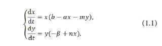
Predator-prey interaction is one of the most significant phenomena among species [1]. In recent years, many mathematicians and biologists have studied the dynamical behaviors between predator and prey [1], especially using the traditional Lotka-Volterra predator-prey model, which takes the form as follows:
Thanks to the pioneering work of Lotka and Volterra, the study of practical mathematical models in ecology has become a hot topic that has attracted a large number of mathematicians and biologists to join in. In the past few years, many mathematicians have been involved in the dynamical behaviors of predator-prey systems with the theory of dynamical system so that abundent significant results have been yielded [1-6].
In the course of studying the dynamics of predator-prey models, many scholars take into account the effect of the functional response for predator to prey. Yu [7] researched the global asymptotic stability of a predator-prey model with modified Leslie-Gower and Holling-II scheme:
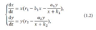
in which x(t)and y(t) denote the densities of the prey and the predator at time t respectively, and are the growth rate of the prey and the predator respectively, r1 and r2measures the strength of competition among the individuals of the prey, a1and2 are the maximum values that per capita reduction rate of the prey and the predator can attain respectively, k1andk2 measure the extent to which the environment provides protections to the prey and the predator respectively [8]. In addition, Yu [7] offered two sufficient conditions on the global asymptotic stability of a positive equilibrium of the system (1.2). After that, Yue [9] considered the dynamics of the following modified Leslie-Gower predator-prey model with Holling-II scheme and a prey refuge:
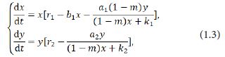
where mx denotes the part of the refuge protection of the prey, and m∈[0,1] . Yue [9] also found that an increase of the amount of refuge may guarantee the coexistence and attractivity of the two species with no difficulty.
Nowadays, cannibalism, a special phenomenon in nature [10-12], has attracted scholars’ attetion, which means the behavior of consuming the same species. Many species in biology have the phenomenon of cannibalism. For example, some mature organisms eat young individuals, and the stronger ones prey on the weaker ones, etc.. Cannibalism occurs in fish, bird and insect, such as Atlantic salmon, red backed spiders and some copepods [10-12]. Due to the need of energy acquisition and others, the behavior of cannibalism will be widely followed in the whole population [10-12]. This strategy helps adult individuals to preserve energy. Cannibalism of biological species will be helpful to the sustainable survival of organisms to a certain extent. It is universally acknowledged that cannibalism has a quite important effect on the dynamical behaviors of the species.
Scholars once used the bilinear function βxy to describe the cannibalism (refer to [10-16] and the references therein). Till recently the thought of the functional response of predator-prey models was adopted [17-18], and the nonlinear cannibalism model was then proposed.
In 2016 Basheer et al. [17] proposed the predator-prey model with nonlinear prey cannibalism in the following form:
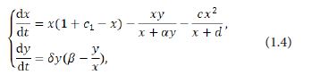
where and represent the densities of prey and predator at time respectively, and the parameters c, c1,α,β,δ and are nonnegetive constants. Unlike the previous works [13-16], Basheer et al. [17] described the cannibalism in the Holling-II type functional response. The general cannibalism term is C(x)=c.x.x/x+a in the prey equation, in which is the cannibalism rate. This term C(x) is manifestly more appropriate to the reality of ecology and has obvious addition of energy to the cannibalistic prey. The addition leads to an increase in reproduction in the prey by adding a term c1 to the prey equation. Apparently c1 < c, as the cannibals need to ingest a lot of prey to produce a new offspring [19]. Scholars concluded that prey cannibalism changes the dynamics of the predator–prey model. The system (1.4) is stable without cannibalism, while it’s unstable with prey cannibalism in the same conditions [17]. After that, Basheer et al. [18] studied the prey-predator model with cannibalism in both predator and prey population and got more comprehensive results.
Model Development
In this paper, we further consider the following predator-prey model with predator cannibalism:
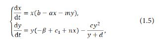
where c1< c. The meanings of parameters in (1.5) are shown in Table 1, and (cy 2/(y+d) denotes the cannibalism of the predator. In biological sense one assumes that all the parameters are nonnegetive constants.
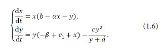
Without loss of generality, we can assume m=n=1 in the system (1.5). In fact, to do this, the transformation (nx,my,md,α/n)→(x,y,d,α) is sufficient. That is to say, in the sequel, we consider the dynamical properties for the following system:
In general, it is of little possiblility to obtain an exact solution for a complex differential equation or system, so we usually derive its appropriate solution by computer. Thus we should study the corresponding discrete model. For a given differential system, many discretization methods can be utilized, including Euler backward difference method, Euler forward difference method and semidiscretization method, etc.. In this paper, we use the semidiscretization method to derive the discrete model of the system (1.6). For the semidiscretization method, refer also to [20-22, 26-29].
For this purpose, firstly suppose that [t] represents the greatest integer not exceeding t. Then consider the average rate of change of the system (1.6) at integer number points in the following form:
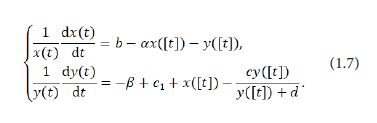
It is quite straightforward to see that piecewise constant arguments occur in the system (1.7) and that any solution (x(t),y(t)) of (1.7) for t∈[0,+∞) is in possession of the following three characteristics:
1.x(t) and y(t) are continuous on the interval [0,+∞);
2.(dx(t))/dt and (dy(t))/dt exist anywhere when t∈[0,+∞) except for the points t∈{0,1,2,3,⋯};
3.the system (1.6) is true in each interval [n,n+1) with n=0,1,2,3,....
The following system can be obtained by integrating the system (1.7) over the interval [n,t] for any t∈[n,n+1) and n=0,1,2,...:
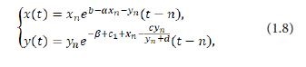
where x_n=x(n) and yn=y(n).Letting t→(n+1)- in the system (1.8) leads to
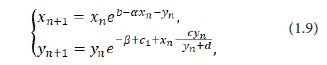
where all the parameters b,c,c_1,d,α,β>0.
In this paper, our main aim is to consider the dynamics properties of the system (1.9), primarily for its stability and bifurcation. We always assume the space of parameters Ω={(b,c,c_1,d,α,β)∈R+6|c1< c}.
The rest of this paper is organized as follows: In Section 2, we discuss the existence and stability of the fixed points of the system (1.9). In Section 3, we derive the sufficient conditions for the occurence of the transcritical bifurcation of the system (1.9). In Section 4, we make some conclusions and discussions about the system (1.9).
Existence and Stability of Fixed Points
In this section, we first consider the existence of fixed points and then analyze the local stability of each fixed point of the system (1.9).
The fixed points of the system (1.9) satisfy
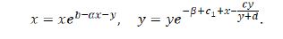
Considering the biological meanings of the system (1.9), we only take into consideration its nonnegative fixed points. Thus, the system (1.9) has and only has four nonnegative fixed points E0 (0,0), E1 (b/α,0), E2 (0,(d(c_1-β))/(β+c-c_1 )) for β< c 1< β+c, and E* (x*,y*) where
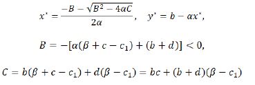
for B2≥4αC and x*< b/α. For the existence of E* (x*,y*), one can also refer to the discussions in its corresponding continuous system in [19].
The Jacobian matrix of the system (1.9) at any fixed point E(x,y) takes the following form
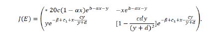
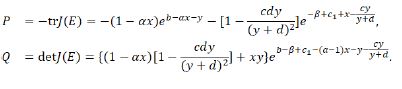
The characteristic polynomial of Jacobian matrix J(E) reads
F(λ)=(λ)2+Pλ+Q,where
Before we analyze the fixed points of the system (1.9), we recall the following lemma [20-22, 26-29].[lem:201]Let F(λ)=λ2+Pλ+Q, where P and Q are two real constants. Suppose λ1 and λ2 are two roots of F(λ)=0. Then the following statements hold.
(i) If F(1)>0, then
(i.1) |λ1 |<1 and |λ2 |<1 if and only if F(-1)>0 and Q<1;
(i.2) λ1=-1 and λ_2≠-1 if and only if F(-1)=0 and P≠2;
(i.3) |λ1 |<1 and |λ2 |>1 if and only if F(-1)<0;
(i.4) |λ_1 |>1 and |λ_2 |>1 if and only if F(-1)>0 and Q>1;
(i.5) λ1 and λ_2 are a pair of conjugate complex roots with |λ1 |=|λ2 |=1
if and only if -2< P<2 and Q=1;
(i.6) λ1=λ2=-1 if and only if F(-1)=0 and P=2.
(ii) If F(1)=0, namely, 1 is one root of F(λ)=0, then the other root λ
satisfies |λ|=(<,>)1 if and only if |Q|=(<,>)1.
(iii) If F(1)<0, then F(λ)=0 has one root lying in (1,∞). Moreover,
(iii.1) the other root λ satisfies λ<(=)-1 if and only if F(-1)<(=)0;
(iii.2) the other root -1< λ<1 if and only if F(-1)>0.
For the stability of fixed points E0 (0,0), E 1 (b/α,0) and E2 (0,(d(c_1-β))/(β+c-c_1 )), we can get the following Theorems 2.2-2.4, respectively.
[theorem:202] The following statements about the fixed point E_0 (0,0) of the system (1.9) are true.
- If β>c1, then E_0 is a saddle.
- If β=c1, then E_0 is non-hyperbolic.
- If β< c1, then E_0 is a source.
Proof. The Jacobian matrix of the system (1.9) at the fixed point E0 (0,0) is given by
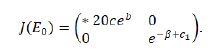
Obviously,λ1=eb > 1 and λ2= e-β+c1 . If β>c1,then , so is a saddle; if β=c1,then |λ2| =1 ,so Eo is non-hyperbolic; if β< c1,then |λ2|>1,so Eo is a source. The proof is over.
[theorem:203] The following statements about the fixed point E1(a/b, 0) of the system (1.9) are true.
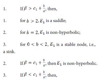
- for b >2, E1 is an unstable node, i.e., a source;
- for b=2, E1 is non-hyperbolic;
- for 0 < b <2, E1 is a saddle.
Proof. The Jacobian matrix of the system (1.9) at E1(a/b, 0) is
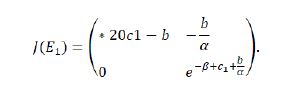
We know λ1 =1-b and λ2=e -β+c1+b/a explicitly.
If β> c1+b/a,then |λ2|<1, so we can get the following results:When b>2,|λ1|>1,so E1 is a saddle;when b=2,|λ1|=1,which says E1 is non-hyperbolic;when 0< b<=2,|λ1|<1,reading E1 is a sink.
If β> c1+b/a,then|λ2|=1,so is non-hyperbolic.
If β> c1+b/a,|λ2|>1 then.Hence,when b>2,|λ1|>1,so E1is a source;when b=2,|λ2|=1, therefore,E1is non-hyperbolic;when 0< b<2,|λ1|<1 ,implying E1 is a saddle.
The proof is complete.
[theorem:204] When β< c1< β+c, E2 (0,(d(c1-β))/(β+c-c1 )) is a nonnegative fixed point of the system (1.9). Let c2 ≜(b+d)/b(c_1-β), c3≜((c1-β)2)/(c1-β-2), and d0≜(2(b+d))/d, then the results about the fixed point E2 of the system (1.9) are summarized in Table 2.
Proof. The Jacobian matrix of the system (1.9) at the fixed point E2 can be simplified as follows:
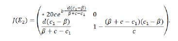
Hereout we obtain λ1=e(b-(d(c_1-β))/(β+c-c_1 )) and λ2=1-((β+c-c1)(c1-β))/c. Therefore,
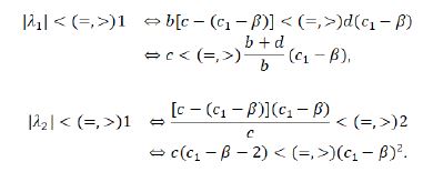
Since β< c1< β+c, here come two cases as follows.
If c≤2, then β< c1< β+c≤β+2, so 0< c1-β<2, which says that c(c1-β-2)<0<(c1-β)2, and hence |λ2 |<1 holds under all circumstances. Therefore, c<(=,>)(b+d)/b(c1-β)≜c_2⇔E_2 is a stable node (non-hyperbolic, a saddle).
If c>2, then, for β< c1≤β+2, c(c1-β-2)≤0<(c1-β)2. So, |λ2 |<1. The type of E2 is determined by the relation |λ1 |<(=,>)1 (hence c<(=,>)c_2). For β+2< c1< β+c,|λ2 |<(=,>)1⇔c<(=,>)((c1-β)2)/(c1-β-2)≜c3.
Furthermore, one can see
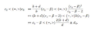
Thereout, we can summarize all the results discussed above in Table 2.
The proof is totally finished.
Bifurcation Analysis
In this section, we use the center manifold theorem and bifurcation theorem to analyze the local bifurcation problems of the fixed points E0 (0,0), E1 (b/α,0) and E2 (0,(d(c_1-β))/(β+c-c_1 )) of the system (1.9). For related bifurcation analysis work for biological systems, refer to the references [26-29] and the references cited therein.
for the Fixed Point E0(0,0)
Theorem 2.2 shows that a bifurcation of the system (1.9) may occur at the fixed point E0 in the space of parameters Ω={(b,c,c1,d,α,β)∈R+6|c1< c} for β=c1. We have the following result.
[theorem:301] Consider the parameters (b,c,c1,d,α,β) in the space Ω. Let β0=c1, then the system (1.9) may undergo a 1:1 strong renonance bifurcation at the fixed point E0 when the parameter β varies in a small neighborhood of the critical value β0.
Proof. We draw the conclusion through the following analysis.
Giving a small perturbation β*=β-β0 with 0<|β*|<<1 of the parameter β, the system (1.9) is perturbed into
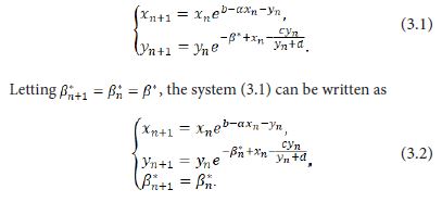
Taylor expanding of the system (3.2) at (xn,xn,βn*)=(0,0,0) takes the form
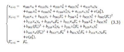
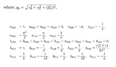
Let
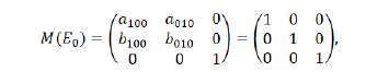
then we derive the three eigenvalues of M(E0) to be λ1,2,3=1, which displays that a 1:1 strong renonance bifurcation may occur at E0(0,0). This will be reserved in the futhur discussion.
For the Fixed Point E1(b/α,0)
Theorem 2.3 shows that a bifurcation of the system (1.9) may occur at the fixed point E1 (b/α,0) in the space of parameters
Ω1={(b,c,c1,d,α,β)∈Ω|β>c1+bn/α}
or
Ω2={(b,c,c1,d,α,β)∈Ω|β< c1+bn/α}
for b=2. Next one will consider these two cases.

In this case, one has the following result.
[theorem:302] Assume the parameters (b,c,c1,d,α,β)∈Ω_1. Let b0=2, then the system (1.9) may undergo a fold-flip bifurcation at the fixed point E1 when the parameter b varies in a small neighborhood of the critical value b0.
Proof. Transform the fixed point E1 (b/α,0) to the origin O(0,0). Giving a small perturbation b*=b-b0 with 0<|b* |≪1 of the parameter b, the system (1.9) is perturbed into
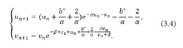
Letting b(n+1)*=bn*=b*, the system (3.4) can be written as
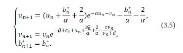
Taylor expanding of the system (3.5) at (un,vn,βn*)=(0,0,0) obtains
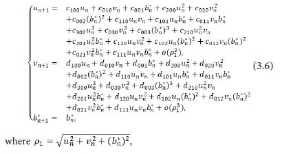
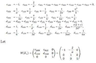
then we derive the three eigenvalues of M(E1) to be λ1=-1 and λ2,3=1. A fold-flip bifurcation may occur at E1 (b/α,0) when b varies in the neighborhood of the critical value b0. This will be focused on our further study.
Case II: b0=2,β< c1+b/α
In this case, one has the following result, whose proof is similiar to the above Subsection 3.2.1 Case I and omitted here.
[theorem:303] Suppose the parameters in Ω2. Put b0=2. Then the system (1.9) may undergo a fold-flip bifurcation at the fixed point E1 when the parameter b varies in a small neighborhood of the critical value b0.
For the fixed point E2 (0,(d(c1-β))/(β+c-c1))
Theorem 2.4 shows that a bifurcation of the system (1.9) may occur at the fixed point E2 (0,(d(c1-β))/(β+c-c1 )) when the parameters occur in the spaces Ω_i,i=3,4,...,7 in Table 3, which can be classified into two cases: one is that the parameter c is perturbed around the critical value c2, and the other is that the parameter c is perturbed around the critical value c3.
Case I: c0=c2
One has the following result.
[theorem:304] Assume the parameters (b,c,c1,d,α,β)∈Ω_i,i=3,4,5,6,7 in Table 3. Let c0=c2=(b+d)/b(c1-β). If (d(c1-β))/(b(b+d))≠2, then the system (1.9) undergoes a transcritical bifurcation at the fixed point E2 when the parameter c varies in a small neighborhood of the critical value c0.
Proof. For convenience of statement, here we take the space of parameters Ω_3={(b,c,c1,d,α,β)∈Ω|c≤2,β< c1< β+c} in Table 3 as an example of verification. The proof for parameters in the other spaces is similar and omitted. The proof of this proposition is based on the following analysis.
Take the changes un=xn-0 and vn=yn-(d(c1-β))/(β+c-c1 ) to translate the fixed point E2 (0,(d(c1-β))/(β+c-c1 )) into the coordinate origin, and the system (1.9) to
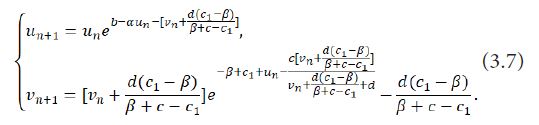
Giving a small perturbation c* of the parameter c, i.e., c*=c-c0=c-c2, with 0<|c* |<<1, the system (3.7) is perturbed into
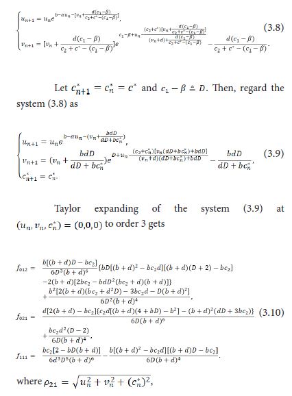
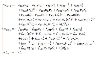
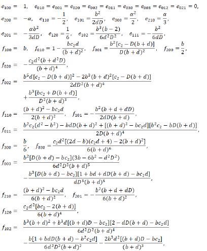
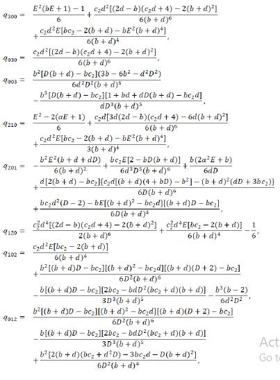
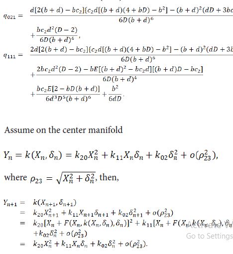
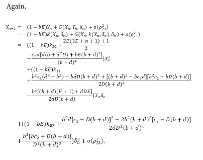
Comparing the corresponding coefficients of terms with the same orders in the above center manifold equation, we get
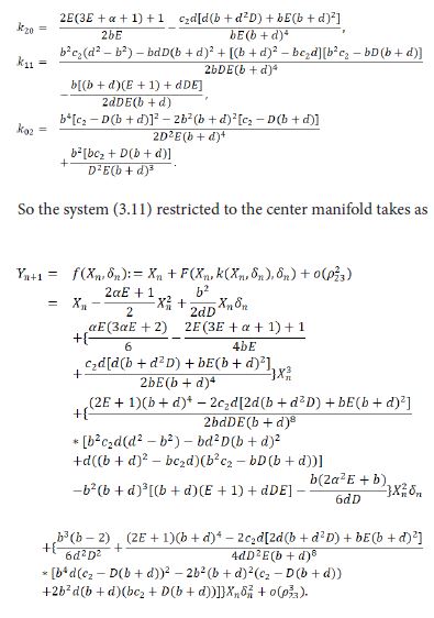
Thereout we have
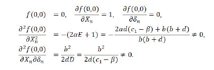
Then, according to [23, (21.1.42-46), p507] or [24,25], it is valid for the occurrence of a transcritical bifurcation in the system (1.9) at the fixed point E2 (0,(d(c1-β))/(β+c-c1)) when the parameter c is perturbed around the critical value c0=c2=(b+d)/b(c1-β) and (d(c1-β))/(b(b+d))≠2 for its parameters in the space Ω3. Then, a transcritical bifurcation of the system (1.9) at the fixed point E2 takes place. The proof is over.
Case II: c0=c3
Similar to the previous Case I, one can get the following result in this case, whose proof is similar, and hence omitted here.
[theorem:305] Suppose the parameters in the space Ω_5 (or Ω_7) stated in Table 3. Let c0=((c1-β)2)/(c1-β-2),If (d(c1-β)2)/((c1-β-2)(b+d)2)≠2, then the system (1.9) undergoes a transcritical bifurcation at the fixed point E2 when the parameter c varies in a small neighborhood of the critical value c0.
Conclusion
In this paper, we analyse the dynamical behaviors of a discrete Lokta-Volterra predator-prey system with the predator cannibalism. Given the parameter conditions, we completely formulate the existence and stability of three nonnegative equilibria E_0 (0,0), E_1 (b/α,0) and E_2 (0,(d(c1-β))/(β+c-c1)). We also derive the sufficient conditions for the transcritical bifurcation of the system to occur at the fixed points E_2 under variaous different conditions. However, it should be pointed out that the positive equilibria E^* (x^*,y^*) and its complex bifurcations have not been discussed yet, which are worthy being considered in our future study.
Acknowledgements
This work is partly supported by the National Natural Science Foundation of China (61473340), the Distinguished Professor Foundation of Qianjiang Scholar in Zhejiang Province(F703108L02), and the Natural Science Foundation of Zhejiang University of Science and Technology (F701108G14).
Competing interests
The authors declare that they have no competing interests.
Authors’ contributions
All authors contributed equally and significantly in writing this paper. All authors read and approved the final manuscript.
- Berryman (1992) The origins and evolution of predator-prey theory. Ecology. 73: 1530-5.
- F Wu, Y Jiao (2019) Stability and Hopf bifurcation of a predator-prey model. Bound. Value Probl. 129: 1-11.
- S Md, S Rana (2019) Dynamics and chaos control in a discrete-time ratio- dependent Holling-Tanner model. J. Egypt. Math. Soc. 48: 1-16.
- Y Luo, L Zhang, Z Teng, et al. (2020) Global stability for a nonau- tonomous reaction-diffusion predator-prey model with modified Leslie- Gower Holling-II schemes and a prey refuge. Adv. Differ. Equ. 106: 1-16.
- Rodrigo, S Willy, S Eduardo (2017) Bifurcations in a predator–prey model with general logistic growth and exponential fading memory. Appl. Math. Model. 45: 134-47.
- Z Li, M Han, F Chen (2012) Global stability of a stage-structured predator- prey model with modified Leslie-Gower and Holling-type II schemes. Int. J. Biomath. 5: 1250057.
- S Yu (2012) Global asymptotic stability of a predator-prey model with modi- fied Leslie-Gower and Holling-type II schemes. Discrete Dyn. Nat. Soc.; 2012; Article ID 208167.
- M A Aziz-Alaoui, M Daher Okiye (2003) Boundedness and global stability for a predator-prey model with modified Leslie-Gower and Holling-type II schemes. Appl. Math. Lett. 16: 1069-75.
- Q Yue (2016) Dynamics of a modified Leslie-Gower predator-prey model with Holling-type II schemes and a prey refuge. SpringerPlus. 5: 461.
- Walters, V Christensen, B Fulton et al. (2016) Predictions from simple predator-prey theory about impacts of harvesting forage fishes. Ecol. Model. 337: 272-80.
- Petersen, K T Nielsen, C B Christensen, et al. (2010) The advantage of starving: success in cannibalistic encounters among wolf spiders. Behav. Ecol. 21: 1112-7.
- Y Kang, M Rodriguez-Rodriguez, S Evilsizor (2015) Ecological and evolu- tionary dynamics of two-stage models of social insects with egg canni- balism. J. Math. Anal. Appl. 430: 324-53.
- S Gao (2002) Optimal harvesting policy and stability in a stage structured single species growth madel with cannibalism. J. Biomath. 17: 194-200.
- M Rodriguez-Rodriguez, Y Kang (2016) Colony and evolutionary dynamics of a two-stage model with brood cannibalism and division of labor in social insects. Nat. Resour. Model. 29: 633-62.
- L Zhang, C Zhang (2010) Rich dynamics of a stage-structured prey-predator model with cannibalism and periodic attacking rate. Commun. Nonlin- ear Sci. Numer. Simulat. 15: 4029-40.
- F Zhang, Y Chen, J Li (2019) Dynamical analysis of a stage-structuered predator-prey model with cannibalism. Math. Biosci. 307: 33-41.
- Basheer E, Quansah S, Bhowmick, et al. (2016) Prey cannibalism alters the dynamics of Holling-Tanner-type predator-prey models. Nonlinear Dynam. 85: 2549-67.
- Basheer R, D Parshad, E Quansah, et al. (2018) Exploring the dynamics of a Holling-Tanner model with cannibaliam in both predator and prey population. Int. J. Biomath. 11: 1850010.
- H Deng, F Chen, Z Zhu, et al. (2019) Dynamic behaviors of Lotka–Volterra predator–prey model incorporating predator cannibalism. Adv. Differ. Equ. 359: 1-17.
- Wang, X Li (2014) Stability and Neimark-Sacker bifurcation of a semi- discrete population model. J. Appl. Anal. Comput. 4: 419- 35.
- Wang, X Li (2015) Further investigations into the stability and bifurcation of a discrete predator-prey model. J. Math. Anal. Appl. 422: 920-39.
- W Li, X Li (2018) Neimark-Sacker bifurcation of a semi-discrete hematopoiesis model. J. Appl. Anal. Comput.; 2018; 8; 1679-93.
- S Winggins (2003) Introduction to Applied Nonlinear Dynamical Systems and Chaos (2nd Edition). Spring-Verlag; New York.
- YA Kuznestsov (1998) Elements of Applied Bifurcation Theory (3rd Edi- tion). Spring-Verlag; New York.
- HS Steven (2015) Nonlinear Dynamics and Chaos with Applications to Physics; Biology; Chemistry; and Engineering (2nd Edition). Westview.
- W Yao, X Li (2022) Complicate bifurcation behaviors of a discrete preda- tor–prey model with group defense and nonlinear harvesting in prey; Appl. Anal.
- Z Pan, X Li (2021) Stability and Neimark–Sacker bifurcation for a discrete Nicholson’s blowflies model with proportional delay; J. Difference Equa. Appl. 27: 250-60.
- Y Liu, X Li (2021) Dynamics of a discrete predator-prey model with Holling- II functional response; Intern. J. Biomath. 2150068.
- M Ruan, C Li, X Li (2021) Codimension two 1:1 strong resonance bifur- cation in a discrete predator-prey model with Holling IV functional response; AIMS Mathematics. 7: 3150-68.
Table 1
Parameter |
Meaning |
x |
density of the prey at time |
y |
density of the predator at time |
b |
intrinsic growth rate of the prey |
a |
intraspecific competetion of the prey |
m |
strength of intraspecific interaction between the prey and the predator |
β |
death rate of the predator |
c1 |
birth rate from the predator cannibalism |
n |
conversion efficiency of ingested prey into new predators |
Table 1 : Parameters in the system (1.5) and their meanings
table2
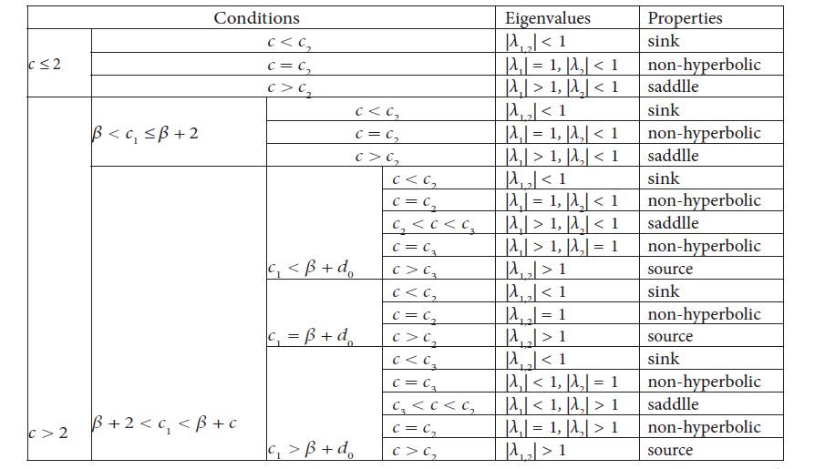
Table 2: Properties of the fixed point E2(0, d(c1-β)/β+c-c1
Tables at a glance