Application of Python Audio Analysis Library for Performing Deep Analysis to Test Signal Homogeneity on an Audio Sample: A Case Study
Received Date: July 07, 2020 Accepted Date: July 24, 2020 Published Date: July 30, 2020
doi: 10.17303/jfrcs.2020.5.102
Citation: Mohit Soni (2020) Application of Python Audio Analysis Library for Performing Deep Analysis to Test Signal Homogeneity on an Audio Sample: A Case Study. J Forensic Res Crime Stud 5: 1-7.
Abstract
This paper proposes a novel method for checking the homogeneity of an audio recording. This case was especially challenging because neither the proper protocols for evidence collection were maintained nor the ‘hash-value’ chain of custody was provided for evidence authentication. Speaker identification was also not a part of the questionnaire and yet the authenticity of the recording was to be established.
The investigation was performed in two steps. Step 1 was a morphological examination of the sample. Step 2 was the step of deep analysis.
py Audio Analysis is a python-based open-source library that calculates thirty-four characteristics from an input sound wave signal, including energy and entropy of energy. The named characteristics were used to mark the signal wave with distinct properties that could help the investigators make a distinction and issue a final decision.
Keywords: Forensic audio analysis; python libraries; the energy of the wave; entropy.
Introduction
This was a case of internal vigilance. A government investigative agency was under the scanner for repeated unproven complaints of bribery. An officer once found himself in the mix of things. He was known to always oppose the routine ways of his office colleagues. His often accused colleagues planned for him an entrapment. A few casually exchanged conversations were captured using a portable mp3 player-cum-voice recorder. Some careful operations later a 22-odd minute audio clip was submitted as evidence against the entrapped officer. This clip had a voice recording of him, asking for money in exchange for unlawful favors.
The case had been contested for several years and had gone through several hearings and rehearing's. After around five years, the entrapped officer was found to be guilty. For the cross-examination of this verdict, the authors' investigation services were sought. All identity revealing details have been omitted since the case is sub judice.
The evidence presented to the authors, for probably the fourth reiteration of cross-examination, was a CD. This CD contained 2 audio files, entitled VOICE001 and VOICE002. These were both in .wav format and had a size of 100 kb and 5 Mb respectively
As stated above, the provided bit of digital evidence is two audio files. File sizes and original creation dates are indicated below in Figure 1.
VOICE001.wav with MD5#449e5f03adif292b19b7580abe995f8d is a recording done in controlled, supervised conditions. It has been used as a control sample for previous speaker identification tests. It is referred to as C. The MD5 value is confirmed and displayed as Figure. 2. C is found to be an audio file in .wav format of duration 00:24 minutes. Its MAC stamp value, original size, and location are depicted as Figure 3.
VOICE002.wav with MD5#ce07d79fa0e24a02f8413d8ef100619b is the questioned voice recording. This is referred to as A. This is depicted below in Figure 4. A is found to be an audio file in .wav format of duration 21:20 minutes. Its MAC stamp value, original size, and location are depicted below, as Figure 5.
The problem assigned was to authenticate the integrity of Sample A considering C as an authentically created control sample.
Investigation and Procedure
The previous cross-examinations had been performed based on the results of speaker identification. The speaker in A was found to match the speaker in control sample C. The question asked from the authors, was to authenticate the homogeneity of the provided sample A, considering C to be a homogenously created control sample. The original mp3 player used to record A was not available anymore. Clearly, A wasn’t the original file created during recording and had been transferred to at least one other device, before burning it onto the optical disk provided. No ‘chain of custody’ or hash values were provided for comparison and authentication. All that existed was a digital file of a recording.
The investigation was broken into two steps. In Step 1, a preliminary manual examination of the provided sample was carried out in its waveform. Audio samples are viewed as a function of frequencies present concerning time [1, 2]. This can be done using any routine sound editing software. Wave Pad Sound Editor Pro, distributed by NCH [3] was employed for this purpose. A screenshot displaying this waveform is given below as Figure 6.
In cases, where doctoring has been performed on an audio clip, it generally refers to editing out clips or adding clips to the main recording. If a new clip is added to the main recording, the junction point of concatenation may be visible. Similarly, if a clip is spliced out of the main recording, the junction point of recombination may be visible. None of these were however found on the morphological waveform examination, performed manually. This does indicate no doctoring but can’t confirm it. Because, in cases where a concatenated/spliced sample is assembled together and then its file format is changed, for example from .mp3 to .wav, these junction points disappear [1]. They can no longer be observed manually. A wasn’t the created file from the original recording device/sensor; this could have been easily done. The outcome of the morphological test done in Step 1 was therefore not found to be effective.
Next, a technique was sought for determining homogeneity. Homogeneity or the lack of it, of an audio wave, may be determined by two possible approaches. First is by determining the sources responsible for producing it. If the recorder used to produce a voice sample is the same throughout and the sample is continuous, one may assume that the recording is homogenous. In cases where the sample has broken but the recorder employed is the same, one may presume that the sample is non-homogenous. But no breaks were observed in Step 1. In contrast, if a sample has been doctored, more than one recording device may have been employed to get the final sample. Then if two different recording devices are found to be employed for creating one sample, one may conclude that the sample is non-homogenous. To understand the second approach, consider a situation where the same recording device has been used to create a sample. A clip recorded at noon in the living room if concatenated with a clip recorded in the evening in the kitchen, using the same recorder, will also then be considered a non-homogenous recording. Therefore, one may conclude that a sample can be considered non-homogenous if either the recording device has been changed or the background-during its creation has been altered.
This hypothesis is not fool-proof as the background can change during the course of a continuous recording as well. But if this happens, it is obvious, that the sample should have an auditory perception attached to such an event. For example, if a conversation occurs near an office window and suddenly a bus passes from below-the the spikes in the frequency graph would indicate additional sudden noise, accompanied by an auditory perception in the recording (sound of the bus).
This paper introduces a fresh technique for performing a test of sample homogeneity. It is referred to as Deep Analysis. This is based on audio processing protocols, as described by Giannakopoulos [4] using a python-based open library for audio signal analysis called pyAudioAnalysis [5, 6]. pyAudioAnalysis offers a variety of audio analysis and processing protocols that involve extensive feature extractions [6]. Feature extraction is a thorough step, of generating feature vectors from an input signal. These feature vectors provide different bits of information regarding the input wave signal. This python-based library is commercially employed by Google and Amazon Voice Assistants, used to classify unknown music samples and categorize them into pre-fed genres and classes [5].
The various feature vectors that are traditionally calculated from an input audio signal, using pyAudioAnalysis are presented below as Table 1. It traditionally calculates thirty-four features from a given wave frame. Out of these 34 feature vectors the author’s utilized feature vector 2 and 3 namely, Energy and Entropy of Energy, for this examination.
Energy is defined as the sum of squares of the signal values normalized by the respective frame lengths. Considering the frame length as constant, energy may be calculated. The entropy of Energy is defined as the entropy of sub-frames’ normalized energies. It can be interpreted as a measure of abrupt changes within a signal, in a particular time frame. These values are integral and a function of time [5].
In Step 2 of the Investigation, a copy of the entire sample was spliced into equal wave frames of 500 milliseconds each. The complete length of sample A is observed to be 21 minutes 20.437 seconds. This translates to a total of 1280.437 seconds. This gives a total of 2561 frames. For convenience, these frames were numbered from A_0 to A_2560, for further processing. Each frame was processed using pyAudioAnalysis and feature vectors were generated. These feature vectors for each frame were stored as a separate array of values. Both steps were repeated with sample C and the obtained values were stored in separate arrays.
Observations
It was observed that a few frames were found to have sudden changes in the value of energy and so high values of entropy. A gradual change in values of entropy is common, over a period of seconds or minutes. But sudden changes in values of entropy, in wave frames of 500 milliseconds only, are an anomaly. The frames found to be possessing anomalous features are presented below in Table 2. Sudden changes in energy can also be associated with sudden loud frequency sounds. So if the high value of entropy is accompanied by an auditory perception in the recording, one may not consider it. The obtained values from sample A were compared to those of Sample C. The relative absence of any sharp changes in the entropy of the wave of Sample C is exactly as per expectations-since sample C is created under controlled conditions.
The values of entropy for all frames have been plotted on a graph. The values corresponding to the wave frames given in (Table 2) are noticeable marked spikes on the otherwise smooth, gradually stepped contour. This graph is displayed in (Figure 7).
The graph for Sample C is just a smooth, gradual, and stepped contour. It is shown in (Figure 8). In a signal wave of continuing conversations, a few frames showing different characteristics may be considered to be an oddity. The wave frames fed as input are real-time recordings and contain both foreground sound and background noise. The peaks are from the high values of entropy observed in wave frames presented in (Table 1). Figure 9 is an indicatory graph of how an altered wave may look like with the spike producing splice, added in.
Inferences
The Voice of a speaker may be mimicked. Noise, however, cannot be forged. Foreground sound may be replicated, but background noise can’t be duplicated [2]. Background noise in a sample is a property of two factors: ambiance and sensor [1]. This means that an audio recording receives noise from the background and the microphone used to record it. In theory, there may be several other minor reasons as well.
Abrupt changes in the values of entropy traditionally occur due to sudden sounds in a recording. On analysis of Sample A, several frames were found to have an abrupt change in the value of entropy which means sudden emergence of sharp frequencies. But there exists no simultaneous auditory perception of these disturbances, in all of them. If the change in energy is the sum total of the energy of sound and the energy of noise, one can say that:
δ𝐸 ∝ (δ𝑆 + δ𝑁)
where δE is changed in energy, δS is changed in sound frequencies and δN is changed in frequencies produced by the noise component. If the sound has no visible change, it may be surmised that noise in the background has changed in the frames in (Table 2).
As per the derived hypothesis in Step 1 of Section 2 of this paper, changes in noise come from either a change in the background of the sound or a change in the microphone used to record the sound. In a homogenous recording, the microphone or background is not liable to change midway through the recording and then revert back to their original state in the following frames. In other words, at points in the signal wave, available as sample A, the energy was found to increase suddenly with no marked change in foreground sounds. This only means the background in these frames changed.
A change in sound cannot be determined here, but a change in noise indicates non-homogeneity in the source of sample A (VOICE002.wav). Determining if the speech in the abnormal micro- frames (stated in Table 2), is mimicked or not, was beyond the scope of this investigation. The source of non-homogeneity could also not be determined based on the available evidence.
Due to the uniqueness of the case, only a limited sample was available for examination. So, in order to confirm the results, the samples were run through a more conventional method discussed in [7] where researchers have used Ordinary Least Square with Linear Predictive Coding for speaker verification. Using LPC technique, automatic formant extraction was done from audio files in question, sample A and sample C. Then the data from the formants of C was compared to the data from the formants of A. This data was used for statistical analysis (using ANOVA). The results so obtained were found to be consistent with the results previously obtained from the method proposed by the authors in this paper. This can act as a confirmatory test to authenticate the proposed methodology.
Conclusion and Future Scope
The employment of open-sourced python audio processing libraries for processing of digital audio evidence is found to be a novel approach towards forensic audio analysis. The utilization of wave characteristics to point out an anomaly in the input signal wave is performed here. This opens up a variety of possibilities. This also allows an investigator to break free from the limitations of the industry made software meant for processing. It adds an additional paradigm to the capabilities of a researcher. This particular case is still in court and the verdict hangs on several factors. However, the implications the evidence could have had on the outcome were negated.
- Maher R (2018) Principles of Forensic Audio Analysis. Springer International Publishing 34.
- Schuller BW (2013) Intelligent Audio Analysis. Springer International Publishing 121.
- (2019) Wave-pad Audio Editing Software.
- Giannakopoulos T (2015) pyAudioAnalysis: An OpenSource Python Library for Audio Signal Analysis. PLoS ONE 10.
- Djebbar F, Ayad B (2017) Energy and entropy-based features for WAV audio Steganalysis. Journal of Information Hiding and Multimedia Signal Processing 8: 168-181.
- Giannakopoulos T (2018) (github.com/tyiannak/pyAudioAnalysis).
- Machado, Vieira Filho, and de Oliveira (2019) “Forensic Speaker Verification Using Ordinary Least Squares,” Sensors 19: 4385.
FIGURE 1
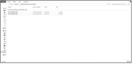
Figure 1: Original Credentials of Evidence
FIGURE 2
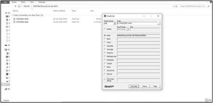
Figure 2: MD5 of Sample C
FIGURE 3
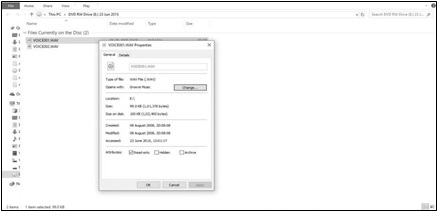
Figure 3: MAC values for Sample C
FIGURE 4
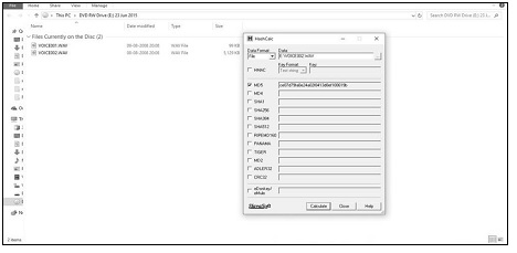
Figure 4: MD5 of A
FIGURE 5
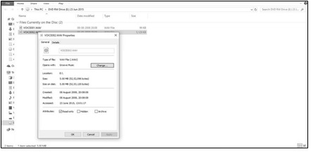
Figure 5:MAC values for A
FIGURE 6
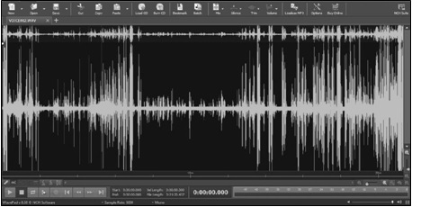
Figure 6:Sample A in the waveform
FIGURE 7
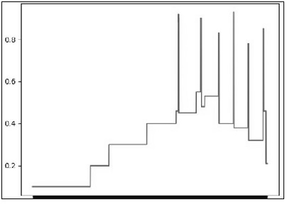
Figure 7:Graph indicating peaks in Energy Curve
FIGURE 8
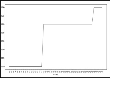
Figure 8: Energy graph for Control Sample C
FIGURE 9
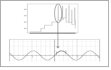
Figure 9:Indicatory representation of suspected addition in wave causing a spike
Tables at a glance