Signal Processing Techniques for Removing Noise from ECG Signals
Citation:Rahul Kher (2019) Signal Processing Techniques for Removing Noise from ECG Signals. J Biomed Eng 1: 1-9.
Electrocardiogram (ECG) is a signal that describes the electrical activity of the heart. The ECG signal is generated by contraction (depolarization) and relaxation (repolarization) of atrial and ventricular muscles of the heart. The ECG signal contains- a P wave (due to atrial depolarization), a QRS complex (due to atrial repolarization and ventricular depolarization) and a T wave (due to ventricular repolarization). A typical ECG signal of a normal subject is shown in (figure 1). In order to record an ECG signal, electrodes (transducers) are placed at specific positions on the human body. Artifacts (noise) are the unwanted signals that are merged with ECG signal and sometimes create obstacles for the physicians from making a true diagnosis. Hence, it is necessary to remove them from ECG signals using proper signal processing methods. There are mainly four types of artifacts encountered in ECG signals: baseline wander, powerline interference, EMG noise and electrode motion
Baseline wander or baseline drift is the effect where the base axis (x-axis) of a signal appears to ‘wander’ or move up and down rather than be straight. This causes the entire signal to shift from its normal base. In ECG signal, the baseline wander is caused due to improper electrodes (electrode-skin impedance), patient’s movement and breathing (respiration). Figure 2 shows a typical ECG signal affected by baseline wander.
The frequency content of the baseline wander is in the range of 0.5 Hz. However, increased movement of the body during exercise or stress test increase the frequency content of baseline wander. Since the baseline signal is a low frequency signal therefore Finite Impulse Response (FIR) high-pass zero phase forward-backward filtering with a cut-off frequency of 0.5 Hz to estimate and remove the baseline in the ECG signal can be used [3].
The presence of muscle noise represents a major problem in many ECG applications, especially in recordings acquired during exercise, since low amplitude waveforms may become completely obscured. Muscle noise is, in contrast to baseline wander and 50/60 Hz interference, not removed by narrowband filtering, but presents a much more difficult filtering problem since the spectral content of muscle activity considerably overlaps that of the PQRST complex. Since the ECG is a repetitive signal, techniques can be used to reduce muscle noise in a way similar to the processing of evoked potentials. Successful noise reduction by ensemble averaging is, however, restricted to one particular QRS morphology at a time and requires that several beats be available. Hence, there is still a need to develop signal processing techniques which can reduce the influence of muscle noise [4]. Figure below shows an ECG signal interfered by an EMG noise.
Electromagnetic fields caused by a powerline represent a common noise source in the ECG, as well as to any other bioelectrical signal recorded from the body surface. Such noise is characterized by 50 or 60 Hz sinusoidal interference, possibly accompanied by a number of harmonics. Such narrowband noise renders the analysis and interpretation of the ECG more difficult, since the delineation of low-amplitude waveforms becomes unreliable and spurious waveforms may be introduced. It is necessary to remove powerline interference from ECG signals as it completely superimposes the low frequency ECG waves like P wave and T wave. (Figure 3) shows an ECG signal typically affected by a powerline interference.
Electrode motion artifacts are mainly caused by skin stretching which alters the impedance of the skin around the electrode. Motion artifacts resemble the signal characteristics of baseline wander, but are more problematic to combat since their spectral content considerably overlaps that of the PQRST complex. They occur mainly in the range from 1 to 10 Hz. In the ECG, these artifacts are manifested as large-amplitude waveforms which are sometimes mistaken for QRS complexes.
Electrode motion artifacts are particularly troublesome in the context of ambulatory ECG monitoring where they constitute the main source of falsely detected heartbeats. A typical ECG signal affected by electrode motion artifact is shown in (Figure 5) below.
In this section, various signal processing methods for removing the artifacts from ECG signal have been described. These methods are simple yet effective. The section also includes the Matlab programs along with their results for the described methods.
A straightforward approach to the design of a filter is to choose the ideal high-pass filter as a starting point [4],
Where, 2cfπ= 2cfπ and sff= sff. Thus, if sf= 0.5 Hz and sf=250 Hz then corresponding normalized cut-off frequency (cf) = 0.002. Since the corresponding impulse response has an infinite length,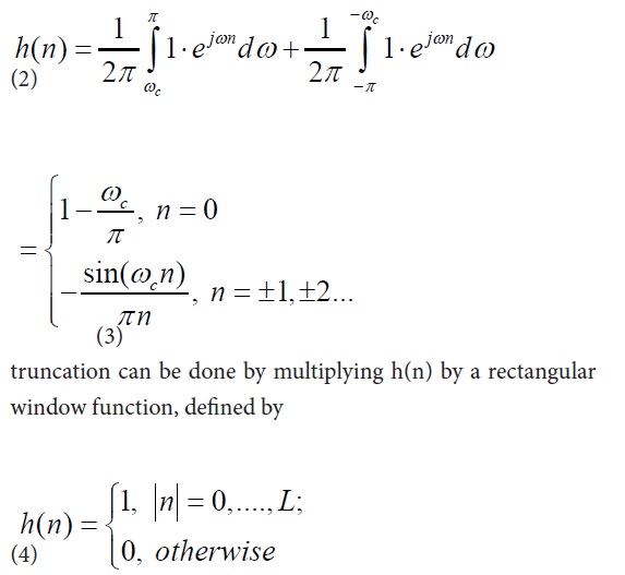
or by another window function if more appropriate. Such an FIR filter should have an order 2L + 1 of approximately 1150 to achieve a reasonable trade-off between stopband attenuation (at least 20 dB) and the width of the transition band.
Matlab code to remove baseline wander using high-pass filter clear all
Fs = 360; % Sampling Frequency
N = 50; % Order
Fc = 0.667; % Cutoff Frequency
% Construct an FDESIGN object and call its BUTTER method.
h = fdesign. lowpass ('N,Fc', N, Fc, Fs);
Hd = butter(h);
x=load('100.txt'); % load the ECG signal
x1=x(:,2);
x2=x1./ max(x1);
subplot (2,1,1), plot(x2), title ('ECG Signal with low-frequency (baseline wander) noise'), grid on
y0=filter (Hd, x2);
subplot (2,1,2), plot(y0), title ('ECG signal with baseline wander REMOVED'), grid on
Wavelet transform can also be used to remove the baseline wander from ECG signal. The frequency of baseline wander is approximately 0.5 Hz. According to discrete wavelet transform (DWT), the original signal is to be decomposed using the subsequent low-pass filters (LPF) and high-pass filters (HPF). The cut-off frequency for LPF and HPF will be half of the sampling frequency. For example, if the sampling frequency is 250 Hz, then 125 Hz will be the cut-off frequency for both LPF and HPF in the first level decomposition. In second level decomposition, the cut-off frequency becomes 62.5 Hz, for third level decomposition it becomes 31.25 Hz and so on. Thus, it will require nine- level decomposition using DWT to remove a baseline wander of 0.5 Hz frequency. Following is the Matlab code to remove baseline wander from an ECG signal using DWT.
Matlab code to remove baseline wander using DWT
x=load ('100.txt');
x1=x (:,2);
x2=x1. /1000;
x2=x2 (170000:215000);
subplot (2,1,1), plot(x2), title ('ECG Signal with baseline wander'), grid on
[C, L] = wavedec (x2,9,'bior3.7'); % Decomposition
a9 = wrcoef ('a', C, L,'bior3.7',9); % Approximate Component
d9 = wrcoef ('d', C, L,'bior3.7',9); % Detailed components
d8 = wrcoef ('d', C, L,'bior3.7',8);
d7 = wrcoef ('d', C, L,'bior3.7',7);
d6 = wrcoef ('d', C, L,'bior3.7',6);
d5 = wrcoef ('d', C, L,'bior3.7',5);
d4 = wrcoef ('d', C, L,'bior3.7',4);
d3 = wrcoef ('d', C, L,'bior3.7',3);
d2 = wrcoef ('d', C, L,'bior3.7',2);
d1 = wrcoef ('d', C, L,'bior3.7',1);
y= d9+d8+d7+d6+d5+d4+d3+d2+d1;
subplot (2,1,2), plot(y), title ('ECG Signal after baseline wander REMOVED'), grid on
A very simple approach to the reduction of powerline interference is to consider a filter defined by a complex-conjugated pair of zeros that lie on the unit circle at the interfering frequency 01,2jzeω±=[4],
Since this filter has a notch with a relatively large bandwidth, it will attenuate not only the powerline frequency but also the ECG waveforms with frequencies close to0ω. It is, therefore, necessary to modify the filter in (6) so that the notch becomes more selective, for example, by introducing a pair of complex-conjugated poles positioned at the same angle as the zeros 01,2jpreω±= but at a radius r,
p,1,2=r±eω
Where 0< r< 1. Thus, the transfer function of the resulting IIR filter is given by
The notch bandwidth is determined by the pole radius r and is reduced as r approaches the unit circle. Figure 8 shows the impulse response and the magnitude function for two different values of the radius, r = 0.75 and 0.95. From Figure 8 it is obvious that the bandwidth decreases at the expense of increased transient response time of the filter. The practical implication of this observation is that a transient present in the signal causes a ringing artifact in the output signal. For causal filtering, such filter ringing will occur after the transient, thus mimicking the low-amplitude cardiac activity that sometimes occurs in the terminal part of the QRS complex, i.e., late potentials [4].
Clear all
Fs = 360; % Sampling Frequency
Fnotch = 0.67; % Notch Frequency
BW = 5; % Bandwidth
Apass = 1; % Bandwidth Attenuation
[b, a] = iirnotch (Fnotch/ (Fs/2), BW/(Fs/2), Apass); Hd = dfilt.df2 (b, a);
x=load ('100.txt'); x1=x (:, 2); x2=x1. / max(x1); Subplot (3, 1, 1), plot(x2), title ('ECG Signal with baswline wander'), grid on
y0=filter (Hd, x2); Subplot (3, 1, 2), plot(y0), title ('ECG signal with low-frequency noise (baswline wander) Removed'), grid on
Fnotch = 60; % Notch Frequency BW = 120; % Bandwidth Apass = 1; % Bandwidth Attenuation
[b, a] = iirnotch (Fnotch/ (Fs/2), BW/ (Fs/2), Apass); Hd1 = dfilt.df2 (b, a);
y1=filter (Hd1, y0); Subplot (3, 1, 3), plot (y1), title ('ECG signal with power line noise Removed'), grid on
The above Matlab code implements two IIR notch filters: one for removing the baseline wander with a notch concentrated at 0.67 Hz and another for removing the powerline interference with a notch concentrated at 60 Hz. The results of the code are shown in (figure 9) below.
The EMG noise is a high-frequency noise; hence an n-point moving average (MA) filter may be used to remove, or at least suppress, the EMG noise from ECG signals. The general form of an MA filter is 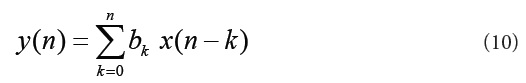
Where x and y are the input and output of the filter, respectively. The bk values are the filter coefficients or tap weights, k = 0, 1, 2, . . . , N, where N is the order of the filter. The effect of division by the number of samples used (N + 1) is included in the values of the filter coefficients. The signal-flow diagram of a generic MA filter is shown in (Figure 10) [5].Increased smoothing may be achieved by averaging signal samples over longer time windows, at the expense of increased filter delay. If the signal samples over a window of eight samples are averaged, we get the output as [5]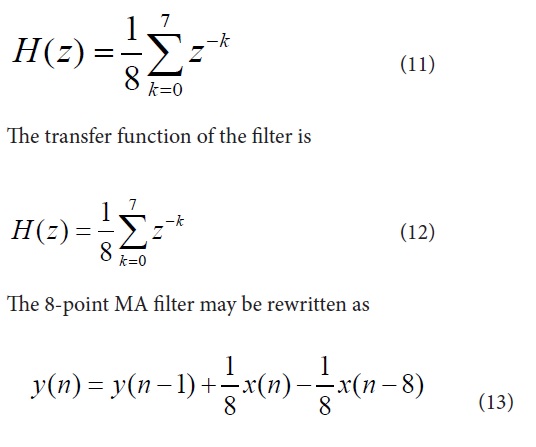
The recursive form as above clearly depicts the integration aspect of the filter. The transfer function of this expression is easily derived to be 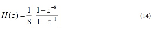
(Figure 11) shows a segment of an ECG signal with high-frequency noise. (Figure 12) shows the result of filtering the signal with the 8-point MA filter described above. Although the noise level has been reduced, some noise is still present in the result. This is due to the fact that the attenuation of the simple 8-point MA filter is not more than -20 dB at most frequencies (except near the zeros of the filter) [5].
Another approach to dealing with this problem is offered by time-varying lowpass filtering using a filter with a variable frequency response. For example, a filter with a Gaussian impulse response has been suggested for this purpose as the filters bandwidth is easily changed from one sample to another through a function (n)β which defines the width of the Gaussian [4],
The width function (n)β is designed to reflect local signal properties so that smooth segments of the ECG are subjected to considerable low-pass filtering, whereas the QRS interval, with its much steeper slopes, largely remains unfiltered. By making (n)β proportional to the derivative of the signal, slow signal changes produce small values of ()nβ, thus making the Gaussian impulse response to decay more slowly to zero so as to produce greater noise suppression, and vice versa. Details of designing the width function(n)β, truncating h (k, n) in (15), and the resulting performance on ECG signals can be found in [5]. The idea of adapting the cut-off frequency of a linear low-pass filter to the slopes of the ECG has also been explored for other types of filters [4, 6 – 8]. For more mathematical details of time-varying filters, references [6 – 9] may be referred.
One of the widely used techniques for removing the electrode motion artifacts is based on adaptive filters. The general structure of an adaptive filter for noise canceling utilized in this paper requires two inputs, called the primary and the reference signal. The former is the d(t) = s(t) + n1(t) where s(t) is an ECG signal and n1(t) is an additive noise. The noise and the signal are assumed to be uncorrelated. The second input is a noise u(t) correlated in some way with n1(t) but coming from another source. The adaptive filter coefficients wk are updated as new samples of the input signals are acquired. The learning rule for coefficients modification is based on minimization, in the mean square sense, of the error signal e(t) = d(t) − y(t) where y(t) is the output of the adaptive filter. A block diagram of the general structure of noise cancelling adaptive filtering is shown in figure 13 [10]. The two most widely used adaptive filtering algorithms are the Least Mean Square (LMS) and the Recursive Least Square (RLS).
Clear all
y1=load ('ECG1.txt'); % this is an ECG signal with motion artifacts
y2= (y1 (:,1)); % ECG signal data a1= (y1 (:,1)); % accelerometer x-axis data a2= (y1 (:,1)); % accelerometer y-axis data a3= (y1 (:,1)); % accelerometer z-axis data
y2 = y2/max (y2); Subplot (3, 1, 1), plot (y2), title ('ECG Signal with motion artifacts'), grid on
a = a1+a2+a3; a=a/max (a);
Mu= 0.0008; Hd = adapt filt. Lms (32, mu); [s2, e] = filter (Hd, a, y2); Subplot (3, 1, 2); plot (s2), title ('Noise (motion artifact) estimate'), grid on
Subplot (3, 1, 3), plot (e), title ('Adaptively filtered/ Noise free ECG signal'), grid on
